
RNA Sequencing Analysis
- Table of Contents
I. Goals
In this section we begin with a broad introduction to the use of RNA deep sequencing towards the goal differential expression testing. This provides the necessary context for the rationale and statistical theory underlying normalization and differential expression testing of RNA sequencing (RNA-seq) data. By then end of this discussion you should:
- Be aware of why RNA-seq data requires normalization
- Understand the rationale behind global normalization
- Be aware of statistical tests used to interrogate differential expression
- Be familiar with the statistical models describing variability in count data
II. Opportunities and challenges
It’s a simple question: What genes are expressed differently between two biological states? In basic research it is common to assess how a treatment modifies expression in vitro relative to controls. In a translational context one often desires to determine how expression evolves over the course of a pathology. While microarrays paved the way for rapid, inexpensive measurements of thousands of transcripts, in the last decade it has been usurped by deep sequencing technologies. As always, RNA-seq technologies come with their unique set of experimental, technical and data analysis challenges.
Using high-throughput sequencing technology to analyze the abundance of RNA species has several advantages over hybridization-based methods such as microarrays (Wang 2009). RNA-seq methods can provide unprecedented insight into alternative splicing, transcriptional initiation and termination, post-transcriptional modification and novel RNA species. From a technical standpoint, the method is unparalleled with respect to measurement noise, sensitivity, dynamic range and reproducibility. The discrete counts arising from sequencing methods are more intuitive than fluorescence intensities. Depending on the conditions, sequencing sensitivity can approach 1 transcript per cell. With great power, however, comes great responsibility.
Normalization
RNA-seq made its debut in the latter-half of the 2000s (Kim 2007) and the hope was, unlike microarrays, it might ‘capture transcriptional dynamics across different tissues or conditions without sophisticated normalization of data sets’ (Wang 2009). As is often the case, a flood of initial excitement and widespread adoption has given way to more nuanced discussions concerning sources of error, bias and reproducibility (Oshlack 2010, Li 2014). Even as late as 2010 a rigorous analysis of methodology had not yet been developed for RNA deep sequencing. Software packages emerging alongside publications have attempted to encapsulate and standardize approaches that control for various sources of ‘error’. Here we expand upon the nature of such errors particularly as they relate to analysis of differential expression.
Statistical models
In practice, assessing differential expression entails a hypothesis test that calculates the probability of an observed difference in RNA species counts between groups/subtypes assuming the null hypothesis of no association between subtypes. Statistical models are introduced into this process in order to provide a more explicit and rigorous basis for modeling variability. Unlike microarrays, which provide continuous measures of fluorescence intensity associated with labelled nucleic acids, deep sequencing produces discrete counts better described by a distinct set of statistical models.
III. RNA sequencing
This section includes a very brief review of RNA-seq concepts and terminology that will be a basis for discussion of data normalization. Many of the TCGA RNA sequencing data sets we describe were generated using the Illumina platform and for that reason we focus on their technology.
A detailed discussion of RNA-seq is beyond the scope of this section. We refer the reader to the RNA-seqlopedia, a rich web resource for all things RNA-sequencing related.
Terminology
Definition A sequencing library is the collection of cDNA sequences flanked by sequencing adaptors generated from an RNA template.
Definition The sequencing depth refers to the average number of reads that align to known reference bases. This concept is also referred to as sequencing coverage.
Definition An aligned read or mapped sequence read refers to a sequencing result that has been unambiguously assigned to a reference genome or transcriptome.
Caution!
The concept of the total number of RNA fragments that are unambiguously mapped to a reference in a given instance of a sequencing workflow is often conflated in the literature with 'library size' and 'sequencing depth'.Sequencing experimental workflow
Figure 1 shows a typical RNA-seq experimental workflow in which an mRNA sample is converted into a set of corresponding read counts mapped to a reference.
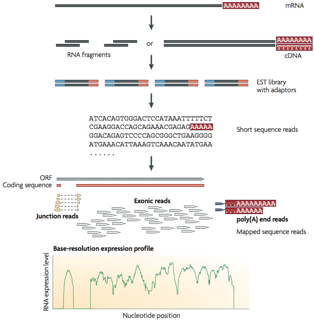
Figure 1. A typical RNA-seq experiment. mRNAs are converted into a library of cDNA fragments typically following RNA fragmentation. Sequencing adaptors (blue) are subsequently added to each cDNA fragment and a short sequence is obtained from each cDNA using high-throughput sequencing technology. The resulting sequence reads are aligned with the reference genome or transcriptome, and classified as three types: exonic reads, junction reads and poly(A) end-reads. These three types are used to generate a base-resolution expression profile for each gene (bottom). Adapted from Wang et al. (2009)
For those more curious about the process by which the short sequence reads are generated, Illumina has made available a summary of their ‘Sequencing by Synthesis’ (SBS) technology.
Sequencing multiple libraries
The workflow described in Figure 1 shows a single sequencing experiment whereby an RNA sample is converted into a cDNA library, sequenced and then mapped to a reference. More often, RNA sourced from distinct biological entities will be sequenced. Figure 2 shows a typical sequencing flow cell consisting of lanes in which samples can be loaded and sequenced in parallel. Correcting for bias between different sequencing experiments will be an important aspect of normalization.
Note: We will use the term ‘sample’ and ‘case’ interchangeably to refer to an a distinct source of biological material from which RNA-seq counts are derived. In each case a cDNA library is created, and so you will often see this concept referred to as a ‘library’.
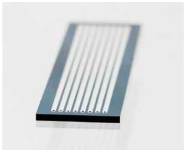
Figure 2. Typical sequencing flow cell apparatus. Several samples can be loaded onto the eight-lane flow cell for simultaneous analysis on an Illumina Sequencing System. Adapted from Illumina Tech Spotlight on Sequencing
IV. Normalization
Variation
RNA-sequencing data is variable. Variability can broadly be divided into two types: ‘Interesting’ variation is that which is biologically relevant such as the differences that arise between cancer subtypes; ‘Obscuring’ variation, in contrast, often reflects the peculiarities of the experimental assay itself and reduces our ability to detect the interesting variation that leads to publications and the envy of colleagues. Obscuring variation in gene expression measurement may be largely unavoidable when it represents random error, such as the stochastic nature of gene expression. In contrast, a large amount of effort has been directed at identifying and attempting to mitigate systematic errors.
Variability obscures comparisons
The path to understanding what underlies a disease pathology or the effect of a drug often begins with determining how they differ from an unperturbed state. In an ideal world we would directly observe those changes. In reality, our observations are indirect and represent inferences upon data that result from many experimental and analysis steps. The aim of normalization is to remove systematic technical effects that occur during data creation to ensure that technical bias has minimal impact on the results.
The overall goal for RNA-seq normalization is to provide a basis upon which an fair comparison of RNA species can be made. The need for normalization arises when we wish to compare different sequencing experiments. In this context, a sequencing experiment is performed on a library created from a single RNA source. Differential expression analysis involves comparing RNA from at least two distinct biological sources, often reflecting different biological states (Figure 3). Moreover, it is common to measure many members of the same type or treated under the same experimental condition. Such ‘biological replicates’ are often used to boost the power to detect a signal between types and average-out minor differences amongst types.
Definition A biological replicate of a set of experiments is performed using material from a distinct biological source.
Definition A technical replicate of a set of experiments is performed using the same biological material.
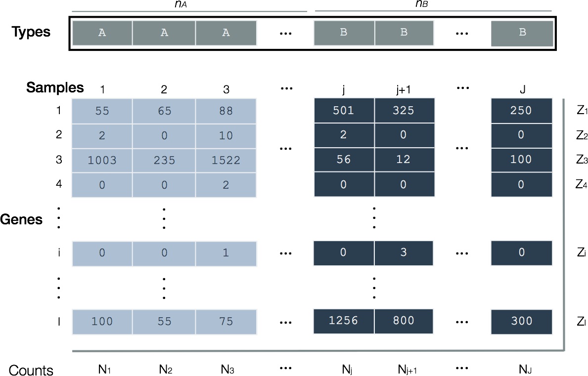
Figure 3. Layout of RNA-seq read counts for differential expression. Hypothetical counts of RNA species for two biological types (A and B) whose gene expression are being contrasted. Samples (J total) are arranged in columns and genes (I total) in rows. There are n_A samples of Type A and n_B of Type B. A cDNA library for each sample is created and sequenced. The total number of mapped sequence reads from each sample (N) are usually non-identical; Total mapped sequence reads for each gene is also indicated along right margin (Z).
Notation
To make our discussion more precise we will use mathematical notation in the following sections.
- observed mapped sequence reads (i.e. fragments or counts) for gene and sample
- = total sample mapped sequence reads in a sample
- = total mapped sequence reads for a gene
- = total mapped sequence reads for a gene over all sample indices corresponding to a given type
- relative abundance of mapped sequence reads attributed to a given locus in a sample. Proportion of total mass
- number of samples of type
- gene expression level in number of transcripts
- length of an RNA species in bases
- total RNA output in a sample. Total mass in bases
- : sample normalization factor
Correction factors
Much of this section is inspired by Ignacio Gonzalez’s tutorial on ‘Statistical analysis of RNA-Seq data’ (Toulouse, November 2014)
We wish to make fair comparisons between RNA sequencing experiments. Such data could arise from sequencing RNA from distinct types (e.g. males and females), the same type (e.g. males; a biological replicate) and perhaps even sequencing the same sample multiple times (e.g. same male; a technical replicate). Here we describe global normalization whereby a correction factor is applied to an entire set of mapped sequence reads (Figure 4).
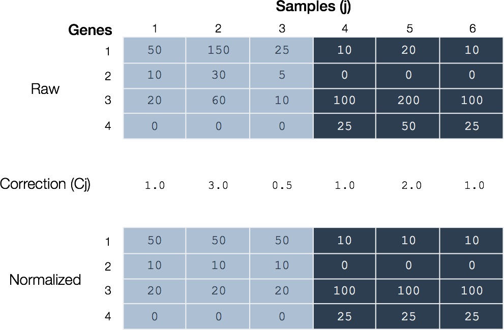
Figure 4. Global normalization. (Above) Hypothetical mapped read counts for samples of two types. Mapped sequence reads for each sample arise from a corresponding cDNA library and sequencing run. (Middle) For each sample (j) a correction factor (Cj) is calculated. In this case, the normalization factor is the ratio of total mapped sequence reads relative to the first of each type (samples 1 and 4). (Below) The normalized data results from dividing mapped sequence reads for each gene by the respective sample correction factor.
Several different normalization schemes have been suggested but which is ‘best’ is an ongoing debate. Here we discuss those relevant to differential expression analysis and available as part of the edgeR Bioconductor package.
Total count
Available in edgeR:
cpm(..., normalized.lib.sizes = TRUE)
In this case, differences in mapped sequence reads for a gene result from variations in sequencing depth. This is the most intuitive scheme: If sample A sequencing results in half the total mapped sequence reads of B, then A will have half the mapped sequence reads of B for any arbitrary mapped RNA species.
This approach can be attributed to Mortazavi et al. (Mortazavi 2008) who claimed ‘The sensitivity of RNA-Seq will be a function of both molar concentration and transcript length. We therefore quantified transcript levels in reads per kilobase of exon model per million mapped reads (RPKM).’
The correction factor is just the sum of mapped read counts for a given sample divided by one million
The ‘kilobase of exon model’ referred to by Mortazavi et al. is necessary to correct for comparison of different species within the same sample. This arises due to the RNA fragmentation step performed prior to library creation: Longer loci generate more fragments and hence more reads. This is not required when comparing the same RNA species between samples such as in differential expression analysis.
Trimmed mean of M-values
Available in edgeR:
calcNormFactors(..., method = "TMM")
Let us consider the rationale underlying total count correction. Strictly speaking, the method rests on the assumption that the relative abundance of RNA species in different samples are identical and that differences in counts reflects differences in total mapped sequence reads.
Of course, there are situations in which these assumptions are violated and total count normalization can skew the desired correction. Consider a scenario where samples express relatively large amounts of an RNA species absent in others (Figure 5). Likewise, consider a situation where a small number of genes in a sample may generate a large proportion of the reads.
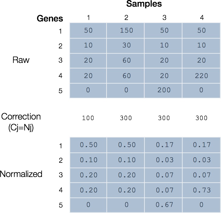
Figure 5. Total count normalization is limited when RNA composition is important. Applying total count normalization to RNA sequencing samples can obscure the true mapped sequence reads for genes in cases where RNA composition is important. Samples 1 and 2 differ only in total mapped sequence reads and are valid under total count normalization. Sample 3 illustrates the case where a sample highly expresses gene 5 that is not otherwise represented. Sample 4 illustrates a case where one gene 4 is highly expressed. Note that in both cases, the result is that genes in samples 3 and 4 are over-corrected.
A more realistic assumption is that the relative expression of most genes in every sample is similar and that any particular RNA species represents a small proportion of total read counts. Robinson and Oshlack (Robinson 2010) formalized this potential discrepancy and proposed that the number of reads assigned to any particular gene will depend on the composition of the RNA population being sampled. More generally, the proportion of reads attributed to a gene in a sample depends on the expression properties of the whole sample rather than merely the gene of interest. In both cases considered in Figure 5, the presence of a highly expressed gene underlies an elevated total RNA output that reduces the sequencing ‘real estate’ for genes that are otherwise not differentially expressed.
To correct for this bias, Robinson and Oshlack proposed the Trimmed mean of M-values (TMM) normalization method. In simple terms, the method makes the relatively safe assumption that most genes are not differentially expressed and calculates an average fold-difference in abundance of each gene in a sample relative to a reference. This average value is the TMM correction factor and is used in downstream analyses to account for differences between sample and reference. A more rigorous description of TMM follows.
TMM notation
Suppose that we observe some number of mapped sequence reads for a gene in a given sample/case/library . The expected value of counts will equal the fraction of the total RNA mass attributed to this RNA species which is the product of the relative abundance multiplied by the total number of mapped sequence reads . Relative abundance is equal to the product of the unknown expression level (number of transcripts) and the RNA species length all divided by the unknown total RNA output in the sample .
It is desirable to calculate the total RNA output as we could use this as our correction factor. However, RNA output is unknown. Instead, we estimate the ratio between sample relative to .
The proposed strategy attempts to estimate this ratio from the data. The assumption is that most genes are expressed at similar levels, then . So we estimate output accordingly:
Note that represents the relative abundance so that the last two terms are the fold-difference between samples. Then define the per-gene log fold-difference
and likewise, the absolute expression levels
Step 1. Trim data
Towards our goal of a robust estimate of total RNA outputs, we remove genes with extreme expression differences beyond a threshold that would skew our estimates. Oshlack and Robinson trim off the upper and lower 30% of and the outer 5% of values. Implicit in the calculation of and is the removal of genes with zero counts.
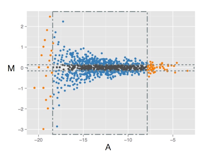
Figure 6. Trimming. Hypothetical RNA sequencing data where per-gene log fold-difference (M) is plotted against absolute expression (A). Thin box (dashed) restricts the data along the vertical axis omitting the outer 30% of values; Large (dashed-dot) box restricts the data along the horizontal axis omitting the outer 5%. Adapted from Ignacio Gonzalez's tutorial on 'Statistical analysis of RNA-Seq data' (Toulouse 2014)
Step 2. Calculate per-gene weights
We could go ahead and simply calculate the mean over all genes. Let us pause a moment and notice in Figure 6 the near universal trend where genes with lower counts (A) have a much wider range of fold-difference (M) and vice versa.
Oshlack and Robinson suggested that to rescue a fairer representation of the mean, those with lower variance should contribute more than those with higher variance. This is the rationale for taking a weighted mean with precision - the inverse of the variance - as weights.
Formally, the weighted mean of a non-empty set of data
with non-negative weights is
Recall the definition of as a log of a ratio, thus exponentiating the weighted mean recovers the original ratio.
-
Aside: Estimating variances via the delta method
The delta method is a statistical procedure used to estimate the variance of a function of a random variable based on an approximation of of the function about its mean value. We will use it to derive an expression for the inverse of the variance, the precision or weights .
Consider an interval containing the point . Suppose that a function with first derivative is defined on . Then by Taylor’s theorem, the linear approximation of for any about is
We will use equality for this relationship moving forward. The expectation of is
Likewise, the variance can be estimated
This is a pretty powerful result. It says that the variance of a function of a variable about the mean can be estimated from the variance of the variable and the squared first derivative evaluated at the mean. Notice that our definition of is a function of observed read counts . Remember our goal:
Now consider just one of the variance terms above. We can use our result for estimating the variance we derived previously
Consider now when the total read counts are relatively large, then the observed read counts is a random variable whose realizations follow a binomial distribution
Let us revisit our variance estimate using the results for binomial distribution in .
If the total read counts are large then we can ignore the constant . Now we are ready to state the estimated variance for the log fold-difference.
Step 3. Calculate the correction
One of the advantages of TMM is that the RNA-seq data themselves are not transformed using the TMM normalization procedure. This leaves the data free from ambiguity and in its raw form. Rather, the correction is applied during differential expression testing by multiplying the total counts or library size by the correction factor resulting in an effective library size used in subsequent analysis steps.
A normalization factor below one indicates that a small number of high count genes are monopolizing the sequencing, causing the counts for other genes to be lower than would be usual given the library size. As a result, the library size will be scaled down, analogous to scaling the counts upwards in that library. Conversely, a factor above one scales up the library size, analogous to downscaling the counts.
- edgeR User Guide, Chapter 2.7.3
V. Differential expression testing
Our goal in this section is to gather evidence that supports a claim that an RNA species is differentially expressed between two types. For illustrative purposes we will refer to contrasting expression in TCGA ovarian cancer subtypes (‘mesenchymal’ vs. ‘immunoreactive’).
Our framework for gathering evidence will be a hypothesis test and the evidence for each gene will be encapsulated in the form of a p-value. Recall that a p-value in this context will be the probability of an observed difference in counts between subtypes assuming no association between expression and subtype exists. This list of p-values for each RNA species will be our goal and represents the raw material for enrichment analysis tools.
Terminology
Suppose that we wish to test whether the relative abundance () of a gene in the set of cases with a HGS-OvCa subtype label ‘mesenchymal’ is different relative to ‘immunoreactive’. Let the set of sample indices belonging to the mesenchymal cases be of which there are cases. Likewise, the set of immunoreactive cases is .
In classic hypothesis testing language, we take the a priori position of the null hypothesis () that the relative abundance is the same in each subtype.
What we wish to do is determine the feasibility of this null hypothesis given our RNA-seq count observations. For any given gene we can summarize our observations in a table (Table 1).
Table 1. Summary of RNA-seq count data

Definition A test statistic is a standardized value that is calculated from sample data during a hypothesis test.
Define the test statistic as the total number of observed mapped sequence reads for the gene of interest over all samples of a subtype.
From this we can state the gene-wise total.
An exact test for 2 types
Our test will determine the exact probabilities of observing the totals for each subtype () conditioned on the sum (). Given equal total mapped sequence reads in each sample we can derive a suitable null distribution (see section ‘Calculating p-values’ below) from which we can calculate a p-value that will support or cast doubt on the . Here, will be a sum of individual probabilities of mapped sequence reads observed (and unobserved).
Let be the joint probability of a given pair of total mapped sequence reads for a given gene over all samples of a given type (e.g. ). Our first restriction is a fixed total . The second restriction is that we only care about those probabilities with value less than or equal to those observed (e.g. ). This corresponds to tables with mapped read count values for a gene more extreme (differentially expressed) hence more unlikely than those observed.
Example
We will reuse an example originally intended to illustrate Fisher’s Exact Test since the concepts are similar. Consider Table 2 which presents a hypothetical table of observed mapped read counts for a gene between our two HGS-OvCa subtypes.
Table 2. Table of observed RNA-seq count data
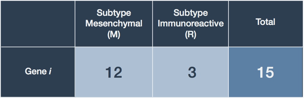
Set marginal totals. Note the marginal read total for the gene is . Given this, our next goal is to enumerate all possible combinations (Table 3).
Table 3. Possible tables given fixed marginal total
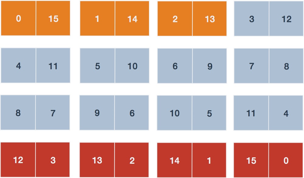
Sum probabilities of contingency tables. If the counts for gene over all samples of each subtype are and , respectively, we desire those table probabilities that are less than or equal to that observed, ). From Table 2 the observed probability is calculated using and giving . Tables highlighted in red include those (unobserved) counts where the gene differential is more extreme than the observed table and consequently will have probabilities lower than the observed. Likewise, tables highlighted in orange will have probabilities lower than that observed. The sum of these two sets of table probabilities will equal .
Calculating p-values
Available in edgeR:
exactTest(...)
Our assumption of independence makes life a little easier in that our joint probability of mapped read counts can be expressed as a product.
Given RNA-seq data samples having the the same total mapped sequence reads (), the probabilities of any particular count can be estimated by a negative binomial distribution.
Here the is the dispersion, is the number of samples of type and is the relative abundance of the gene. But let’s back up a bit. We seemed to pull this negative binomial distribution out of a magic hat. Where does this originate? What do all these parameters really mean and how do we get them?
VI. Modelling counts
Our goal here is to rationalize the negative binomial distribution as an acceptable null probability distribution which we can use to map an observed RNA-seq sequenced read count to a corresponding p-value . In simple terms, trying to derive the null distribution corresponds to the question: How are RNA-seq mapped sequence reads distributed? Another way of stating this is: How do RNA-seq mapped sequence read data vary?
Technical variability
Consider the RNA-seq experiment we presented in Figure 1: RNA is sourced from a particular case, a corresponding cDNA library is generated and short sequence reads are mapped to a reference. Thus, for any give gene we will derive a number of fragment counts. Imagine that we could use the identical cDNA library in multiple, distinct, parallel sequencing reactions such as that provided by a typical flow cell apparatus (Figure 2). Our intuition would lead us to expect that the sequencing reads to be similar but unlikely to produce exactly the same counts for every gene in every reaction.
Definition The technical variability or shot noise is the variability attributed to the nature of the measurement approach itself.
Consider a case where we observe a given number of elements of a given type (e.g. counts of an RNA transcript) within a sample (e.g. all measured transcripts) of elements chosen at random from a population (e.g. expressed transcripts). The probability of any particular is well described by a hypergeometric distribution. The popular example is the probability of consecutive aces when selecting cards without replacement from a standard playing deck . Of course, probabilities are just declarations of our uncertainty. Thus in experimental trials, we expect actual counts to vary about the number prescribed by probabilities.
In practice, hypergeometric probability calculations are expensive and so is approximated by the binomial distribution when the population size is large relative to the sample size .
Two important points about binomial distributions. First, is that it describes a situation in which we have a priori knowledge of the number of observations . In RNA-seq parlance this amounts to knowing the number of mapped RNA species we will observe. Second, the binomial is well-approximated by the Poisson distribution when the sample size is large and the probability of observing any particular species is small. This probability amounts to the relative abundance of a given RNA species.
Modelling the technical variability associated with repeated RNA-seq measurements of a given library with as a Poisson distribution is attributed to Marioni et al. (Marioni 2008).
Statistically, we find that the variation across technical replicates can be captured using a Poisson model, with only a small proportion (∼0.5%) of genes showing clear deviations from this model.
Accordingly, the mean and variance of mapped read counts is a random variable .
A nice aspect of the Poisson distribution is the equality between mean and variance. Figure 7 displays a plot of simulated RNA-seq data where mean and variance for genes is measured across technical replicates.
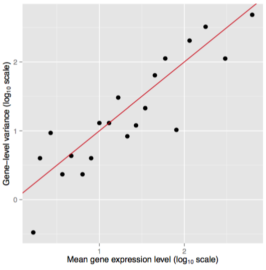
Figure 7. Poisson distributed data. Simulated data showing the relation between mean and variance for technical replicates. The red line shows the variance implied by a Poisson distribution. Adapted from Ignacio Gonzalez's tutorial on 'Statistical analysis of RNA-Seq data' (Toulouse 2014)
Biological variability
Consider the RNA-seq experiments we presented in Figure 3: RNA is sourced from two distinct subtypes and for each subtype, multiple cases. Again, for each case a corresponding cDNA library is generated and short sequence reads are mapped to a reference. Suppose we restrict our attention to cases of a given subtype. Our experience would lead us to expect that the sequencing reads would be similar but unlikely to produce exactly the same counts even after controlling for technical variability.
Definition The biological variability is the variability attributed to the nature of the biological unit or sample itself.
Consider a case where the technical variability in measured counts for a given case/cDNA library is well accounted for by a Poisson distribution indexed by its mean . If we now made our measurements across different cases we would expect additional variability owing to the ‘uniqueness’ of individuals that includes (but not limited to) genetic, physiological and their environmental factors. Figure 8 displays a plot of simulated RNA-seq data where mean and variance for genes is measured across biological replicates.
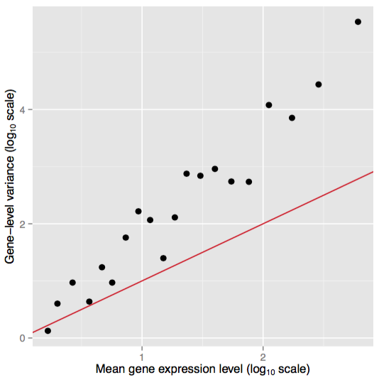
Figure 8. Overdispersed Poisson distributed data. Simulated data showing the relation between mean and variance for biological replicates. The red line shows the variance implied by a Poisson distribution. Adapted from Ignacio Gonzalez's tutorial on 'Statistical analysis of RNA-Seq data' (Toulouse 2014)
The overdispersed count data observed with biological replicates manifests as an elevated variance relative to the mean. Thus, some ‘fudge factor’ is desired to account for this additional variability. The negative binomial arises from a Gamma-Poisson mixture in which a Poisson parameter is itself a random variable and .
Modelling the technical and biological variability associated with RNA-seq measurements of different biological sources as a negative binomial distribution is attributed to Robinson and Smyth (Robinson 2008).
We develop tests using the negative binomial distribution to model overdispersion relative to the Poisson, and use conditional weighted likelihood to moderate the level of overdispersion across genes.
Noise partitioning
The negative binomial as a model of an overdispersed Poisson has the following moments.
Let’s take a closer look at the variance. When the dispersion parameter approaches zero the variance approaches the mean and hence, becomes increasingly Poisson-like. In other words, we might view the negative binomial variance as the sum of two parts: The Poisson-like technical variability and the overdispersion arising from biological (and other inter-sample) sources .
Let’s transform this into a form that you may also see. Dividing each side of the variance by .
Where we have now broken down the total squared coefficient of variation () as a sum of the technical () and biological () squared coefficients of variation. Of course, the biological coefficient of variation may contain contributions from technical sources such as library preparation.
When a negative binomial model is fitted, we need to estimate the BCV(s) before we carry out the analysis. The BCV … is the square root of the dispersion parameter under the negative binomial model. Hence, it is equivalent to estimating the dispersion(s) of the negative binomial model.
VII. Dispersion estimation
Let us preview what we will discuss in this section. Recall in the previous section differential expression testing we defined our test statistics - the number of observed counts for the gene of interest in each subtype.
It turns out that the sum of independent and identically distributed negative binomial random variables is also negative binomial. We snuck this fact into our discussion in the previous section for calculating p-values. In particular, for our HGS-OvCa subtypes
Where is the number of samples of a given subtype. Let us return again to a key assumption that there is a common value for total mapped sequence reads (). This assumption is required as without it, the data is not identically distributed and consequently the distributions of within-condition data totals are not known. Recall again this assumption is unlikely to occur in practice and motivates the adjustments described by Robinson and Smyth (Robinson 2007, Robinson 2008).
Estimating common dispersion
Available in edgeR:
estimateCommonDisp(...)
This is a method suggested by Robinson and Smith (Robinson 2008) who were concerned with a forerunner of RNA sequencing called Serial Analysis of Gene Expression (SAGE). The motivation behind this method is that often times, few biological replicates are available (e.g. less than three). Instead, we leverage the availability of observations across all genes towards the estimation of a common dispersion shared by all genes.
Conditional maximum likelihood (CML)
Suppose once again that represents the observed number of mapped sequence reads for a gene and sample and . Let us restrict ourselves to the set of biological replicates where each sample is from the same condition . In the case that the total mapped sequence reads are equal then their sum
Let us drop the subscripts and assume that we are examining a single gene for samples of a given type. Now it is simple to show that the sample sum is a sufficient statistic for . In this case, we can effectively rid ourselves of in an estimate of by forming a likelihood expression for conditioned on the sum .
In practice we will work with the conditional log-likelihood.
Using the definition of conditional probability we can write.
This is the probability distribution of the counts conditioned on the sum and we will proceed by finding the numerator and denominator separately. To do this, we’ll start with some notation that is simplified by restricting our discussion to a single gene and sample type.
The denominator of the conditional probability distribution is found by recalling that the sum has a negative binomial distribution .
The numerator of the conditional probability is found as usual.
Where the final equality results from us multiplying the numerator and denominator of the fractions by . Then we can take the difference of the two previous results to derive the log-likelihood we are looking for.
Crossing out terms leaves us with the result.
If we ignore terms that do not contain the parameter of interest then we are left with an equation quoted by Robinson and Smyth (Equation 4.1 in Robinson 2008) that we wish to maximize.
Now let us return to our original scenario of multiple samples that fall under one of two conditions . Then for any given gene the conditional likelihood expression expands to encompass both groups.
The commons dispersion estimator maximizes the common likelihood over all genes.
Quantile-adjusted CML (qCML)
The common likelihood we wish to maximize is contingent on equal total mapped sequence reads for each sample, that is, for all . This is pretty unrealistic. As a workaround, Robinson and Smyth devised an iterative algorithm that involves ‘quantile adjustment’ of mapped sequence reads for each gene in each sample into pseudodata that represent the counts that would occur had the total reads been equal to the geometric mean of all samples () (Figure 9A).
It is the pseudodata that is applied to the CML estimate for common dispersion (Figure 9B). In effect, the algorithm adjusts counts upwards for samples having total mapped sequence counts below the geometric mean and vice versa.
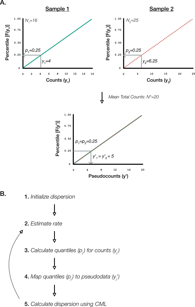
Figure 9. Quantile adjusted conditional maximum likelihood (qCML). A. (Above) Method to map hypothetical counts in two samples to their respective quantiles. In sample 1, there are 16 total mapped sequence reads and so a gene with 4 counts represents the 25th percentile. Likewise, the same gene maps to the 25th percentile for sample 2 that has 25 total counts. (Below) Mapping the 25 percentile in a hypothetical sample with total counts equal to the geometric mean (20) results in equal pseudodata for sample 1 and 2 of 5 counts. B. The qCML algorithm is iterative and uses the pseudodata to calculate the CML over all gene, samples, and sample conditions as described in main text.
Estimating per-gene (‘tag-wise’) dispersions
Available in edgeR:
estimateTagwiseDisp(...)
It can be argued that the dispersion for each gene is different. Consequently, the common dispersion may not accurately represent the count distribution. To account for this, Robinson and Smyth (2007) employed a weighted likelihood
where is a weight given to the common likelihood - the conditional likelihood summed over all genes. Clearly, a relatively large means we revert to using the common dispersion and vice versa. Robinson and Smyth describe the selection of a suitable somewhere between the two extremes. A through discussion of per-gene or ‘tag-wise’ dispersion estimation is beyond the scope of this section. We refer the reader to the original publication by Robinson and Smyth (Robinson 2008) for a detailed discussion of the rationale and approach.
In the end, an estimate of negative binomial parameters enables us to calculate the exact probabilities of RNA-seq mapped read counts and derive a value for each gene, as discussed in the previous section. Dispersion plays an important role in hypothesis tests for DEGs. Underestimates of lead to lower estimates of variance relative to the mean, which may generate false evidence that a gene is differentially expressed and vice versa.
References
- Bullard JH et al. Evaluation of statistical methods for normalization and differential expression in mRNA-Seq experiments. BMC Bioinformatics. 2010 Feb 18;11:94. doi: 10.1186/1471-2105-11-94.
- Conesa A et al. A survey of best practices for RNA-seq data analysis. Genome Biol. 2016 Jan 26;17:13. doi: 10.1186/s13059-016-0881-8.
- Kim JB et al. Polony multiplex analysis of gene expression (PMAGE) in mouse hypertrophic cardiomyopathy. Science. 2007 Jun 8;316(5830):1481-4. doi: 10.1126/science.1137325.
- Li S et al. Detecting and correcting systematic variation in large-scale RNA sequencing data. Nat Biotechnol. 2014 Sep;32(9):888-95. doi: 10.1038/nbt.3000. Epub 2014 Aug 24.
- Marioni JC et al. RNA-seq: an assessment of technical reproducibility and comparison with gene expression arrays. Genome Res. 2008 Sep;18(9):1509-17. doi: 10.1101/gr.079558.108. Epub 2008 Jun 11.
- Mortazavi A et al. Mapping and quantifying mammalian transcriptomes by RNA-Seq. Nat Methods. 2008 Jul;5(7):621-8. doi: 10.1038/nmeth.1226. Epub 2008 May 30.
- Oshlack A et al. From RNA-seq reads to differential expression results. Genome Biol. 2010;11(12):220. doi: 10.1186/gb-2010-11-12-220. Epub 2010 Dec 22.
- Robinson MD & Smyth GK. Moderated statistical tests for assessing differences in tag abundance. Bioinformatics. 2007 Nov 1;23(21):2881-7. doi: 10.1093/bioinformatics/btm453. Epub 2007 Sep 19.
- Robinson MD & Smyth GK. Small-sample estimation of negative binomial dispersion, with applications to SAGE data. Biostatistics. 2008 Apr;9(2):321-32. doi: 10.1093/biostatistics/kxm030. Epub 2007 Aug 29.
- Robinson MD & Oshlack A. A scaling normalization method for differential expression analysis of RNA-seq data. Genome Biol. 2010;11(3):R25. doi: 10.1186/gb-2010-11-3-r25. Epub 2010 Mar 2.
- Wang Z et al. RNA-Seq: a revolutionary tool for transcriptomics. Nat Rev Genet. 2009 Jan;10(1):57-63. doi: 10.1038/nrg2484.